from sklearn.naive_bayes import CategoricalNB
import pandas as pd
import numpy as np

# Importing customer_churn
customer_churn = pd.read_csv("https://raw.githubusercontent.com/Datakortex/Datasets/refs/heads/main/customer_churn.csv")

# Creating column Churn_Label
customer_churn["Churn_Label"] = np.where(customer_churn["Churn"] == 1, "Churn", "No Churn")

# Separating predictors and target variable
X = customer_churn[["Recency_Level", "Frequency_Level", "Monetary_Value_Level"]]
y = customer_churn["Churn_Label"]Naive Bayes
Introduction
Imagine you have just made a subscription to an online movie streaming service, such as HBO or Netflix. Some weeks after your subscription, you have watched 20 movies on this platform, out of which, you liked 15 and disliked the other 5 (in practice, there will be movies where you express no opinion, but let’s assume this is not the case for now). If no other information is available about you, the service could argue that the probability that you like a movie would be 75% (15 / 20). However, what if out of the 15 movies that you liked, 14 of them were suggested by a close friend of yours, with whom it happens that you share similar interests? What if your friend discouraged you to watch the other 5 movies, out of which you liked only one? It is not difficult to understand that, by taking more information into account (e.g., your friend’s suggestion), the estimated probability of you liking the streaming service movies changes. According to the data, if you were to watch a movie that your friend suggested, we would estimate that the probability that you will actually like it would arguably be higher than 75%.
In this chapter, we attempt a short primer on probability essentials as a precursor to one of the most useful machine learning methods for classification, called Naive Bayes. This method is based on the Thomas Bayes’ Theorem which is the basis for conditional probability analysis. The term “naive” comes from the fact that we make a very “naive” assumption, which in reality does not hold in most applications (Lantz, 2023). Nonetheless, this should not discourage us from using this method in practice; we discuss more details about this assumption later in this chapter.
Visiting Probability Theory
Let us revisit the above case of online movie platform subscription. Whether you like or dislike a movie or a series can be thought of as an event for which there are only two possible outcomes: you either like the movie or the TV series, or you may not. In the absence of any additional information, the probability that you actually like any given movie or TV series is represented as:
\[P(\text{Like})\]
In our example, our starting point was that, out of 20 movies, you liked 15. Respectively, the probability that you like any given movie is estimated as \(P(\text{Like}) = 75\%\). Of course, if \(P(\text{Like}) = 75\%\), then \(P(\text{Dislike}) = 25\%\) (remember, the sum of the probabilities of all possible outcomes of an event should always equal 100%). In probability theory, we say that these two outcomes (like a movie and dislike a movie) are mutually exclusive and collectively exhaustive (MECE).
But what if we had additional information? As mentioned in our earlier example, it makes sense to think that the probability that you like a movie on the online platform increases if that movie is recommended by your friend. Things start to become more complicated when we want to calculate the probability of an event based on the probability of (many) other events.
Would the probability of you liking a movie still increase if another event were to happen, such as you flipped a coin and got heads? In probability theory, it is always important to know whether two events are independent or dependent. We say that two events are independent when they are unrelated to each other or the outcome of one does not affect the outcome of the other. For instance, the probability that you like a particular movie is independent from getting heads (or getting tails for that matter) when flipping a coin. The probability that you like a movie is still \(P(\text{Like}) = 75\%\) and the probability that you get heads (assuming that the coin is fair) is \(P(\text{Heads}) = 50\%\). Because these two events are independent, we can only calculate the joint probability that you both like the movie and you get heads. To calculate the probability of two independent events, we simply multiply the probability of one outcome with the probability of the other. Therefore, mathematically, we have:
\[P(\text{Like} \cap\ \text{Heads}) = P(\text{Like}) \times P(\text{Heads}) = 75\% \times 50\% = 37.5\%\]
Thus, the probability for these two outcomes happening simultaneously is 37.5%. Once again, we calculate the probability using the multiplication of individual probabilities because the underlying events are independent.
At this point, it makes sense to ask what changes if two events are dependent. By definition, events would be dependent if the outcome of the one event is related to that of the other. For example, if we know that your friend suggests a movie, the probability that you like the movie is higher, meaning that one event influences the other; the events are not independent. In this case, we are interested in the following probability:
\[P(\text{Like} | \text{FriendSuggests})\] The vertical bar “|” is read as “given”. This mathematical expression is also known as conditional probability and, in the context of this example, it describes the probability that you like a movie given that your friend is suggesting it (or has suggested it) for you to view. If your friend does not suggest the movie, then we would have \(P(\text{Like} | \text{FriendNOTSuggests})\). The other two possible outcomes can be expressed as: \(P(\text{Dislike} | \text{FriendSuggests})\) and \(P(\text{Dislike} | \text{FriendNOTSuggests})\). To understand how we could calculate the \(P(\text{Like} | \text{FriendSuggests})\), we need to have a look at the following frequency table:
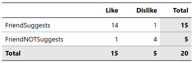
Looking at the first row of this table, we can see that out of the 15 movies that your friend suggested, you liked 14 of them. Therefore, we have:
\[P(\text{Like} | \text{FriendSuggests}) = \frac{14}{15} = 93\%\]
This is a much higher probability because your friend’s recommendations provide additional information about whether you are likely to enjoy a particular movie. The fact that the probability increases in this way reflects the extra information we gain from your friend’s suggestion, which is precisely why the two events are dependent.
The frequency table allows us to calculate conditional probabilities directly by counting observations. However, there is also a general mathematical formula for calculating conditional probabilities. This formula is known as Bayes’ theorem, which expresses the probability of an event using prior information that may be related to that event. In our example, the prior information is whether your friend suggested the movie. Mathematically, Bayes’ theorem can be written as:
\[P(\text{Like} | \text{FriendSuggests}) = \frac{P(\text{FriendSuggests} | \text{Like}) \times P(\text{Like})}{P(\text{FriendSuggests})} = \frac{P(\text{Like} \cap \text{FriendSuggests})}{P(\text{FriendSuggests})}\]
The probability \(P(\text{Like})\) is equal to \(\frac{15}{20}\) because out of the total 20 movies, you liked 15 of them. Notice how this calculation does not take into account any suggestions; it is based on all movies in the table. Similarly, the probability \(P(FriendSuggests)\) is also \(\frac{15}{20}\). Notice that both \(P(Like)\) and \(P(FriendSuggests)\) are calculated using all 20 movies in the dataset. Conditional probability differs because we restrict our attention to a subset of the data—in this case, only movies that were suggested by your friend. In this sense, conditional probability can be interpreted as probability calculation after filtering the data according to some condition. Additionally, the joint probability \(P(\text{Like} ∩ \text{FriendSuggests})\) is equal to \(P(\text{FriendSuggests} | \text{Like}) \times P(\text{Like})\), not to \(P(\text{Like}) \times P(\text{FriendSuggests})\), due to the fact that the events are dependent. Regarding the calculation, we have:
\[P(\text{Like} | \text{FriendSuggests}) = \frac{P(\text{FriendSuggests} | \text{Like}) \times P(\text{Like})}{P(\text{FriendSuggests})} = \frac{\frac{14}{15} \times \frac{15}{20}}{\frac{15}{20}} = 93\%\]
To sum up, when we have independent events (e.g., A and B), we calculate the joint probability using \(P(A ∩ B) = P(A) \times P(B)\), and the order does not matter as the events are independent. However, with two dependent events, we have the following scenarios:
\(P(A∩B) = P(B|A) \times P(A)\)
\(P(B∩A) = P(A|B) \times P(B)\)
Using our previous example, we can imagine that the probability you like the movie, given your friend recommends it, is different from the probability that your friend recommends a movie, given you like it. Thus, when events are dependent, the conditional probability depends on the direction of conditioning. In general, \(P(A|B)\) is not equal to \(P(B|A)\), so the order of the events matters.
Naive Bayes Method
The Thomas Bayes’ formula is the base of the Naive Bayes method in machine learning. Essentially, we can create a model that can be used for prediction, starting from pre-existing (or pre-measured) independent variables. In our movie suggestion example, we saw mathematically how we could incorporate the information regarding your friend’s suggestion to make way more accurate estimations. Without the information about your friend’s suggestion, we saw that the probability you would like a movie would be 75%.
However, things start to become complicated as we include more and more information. For instance, what if we have suggestions from 10 friends instead of just 1? In that case, we would have 10 different events and we would need to calculate all these joint probabilities to apply Bayes’ formula. In other words, it would be too difficult and computationally expensive to apply Bayes’ formula to calculate all these conditional probabilities. Instead, Naive Bayes algorithm makes a very strong, yet “naive” assumption, about the relationships among the events: that all events are independent. We saw earlier that when we calculate independent events, we just multiply each others’ probabilities, without further consideration; indeed, this is how the Naive Bayes algorithm estimates the probability of an observation of interest.
How Naive Bayes Simplifies Bayes’ Theorem
This is somewhat ironic. Although Naive Bayes is based directly on Bayes’ theorem, its practical usefulness comes from the strong independence assumption. The theorem itself remains unchanged; what changes is the calculation of the numerator. Instead of estimating a potentially very complex joint probability such as \(P(X_1, X_2, ..., X_k)\), Naive Bayes assumes that the predictors are independent and approximates this term as \(P(X_1 | Y) \times P(X_2 | Y) \times ... \times P(X_k | Y)\). This dramatically simplifies the calculations and makes Bayes’ theorem computationally feasible even when many predictors are included.
Another adjustment that is needed in Naive Bayes is that of zero probabilities. We need to keep in mind that there might be combinations of events for which the estimated probability is, in fact, zero. For instance, suppose that among all the movies your friend recommended, there was never a single horror movie. If we were to estimate the probability of a movie being a horror movie given that your friend recommended it, we would obtain a probability of 0 based on the observed data.
This creates a problem for Naive Bayes. Recall that the method multiplies many conditional probabilities together, meaning that if even one of these probabilities is equal to 0, the entire product becomes 0, regardless of how strong the evidence from the other variables may be. As a result, a single unobserved combination of events could completely rule out a prediction.
To address this issue, Naive Bayes typically uses Laplace smoothing (also known as the Laplace estimator or add-one smoothing). Instead of assigning a probability of exactly 0 to unseen events, we add a small positive value (usually 1) to each frequency count in the data before converting them into probabilities. In practice, this means we assume that every possible event has at least a very small, non-zero probability. This prevents the numerator in Bayes’ formula from collapsing to zero and ensures that the model can still make meaningful predictions even for combinations of events not observed in the training data.
Assumptions
Naive Bayes employs mainly two assumptions. For one, we discussed how event independence is at the core of this machine learning method while, second, we assume that all events considered are equally important (we do not give a priority to one event over another one). Let us explicitly mention these assumptions below:
Conditional Independence: This is the “naive” part of Naive Bayes. It assumes that the presence (or absence) of a particular feature is independent from the presence (or absence) of other features.
Feature Relevance: All features are relevant and equally important.
In our movie recommendation example, we assume that the recommendation of one friend is independent from the recommendation of all other friends (one’s opinion does not affect and is not affected by the opinion of the others), and that all recommendations are equally important (we do not value any one recommendation more than any other).
Naive Bayes in Python
Let us explore how to use the Naive Bayes method by using the customer_churn dataset, available on GitHub. Using this dataset, we will use the categorical variables Recency_Level, Frequency_Level and Monetary_Value_Level to predict whether a customer churns or not. Additionally, we create the variable Churn_Label, which will have the value "Churn" if the original value of the variable Churn is 1, and the value "Not Churn" if it is 0.
In the code below, we load the necessary library, separate the target variable and predictors, and ensure that the target variable Churn_Label is properly defined, as described earlier.
To keep things simple, we split the dataset into a training and a test set, with 75% (or 3,000 rows) and 25% (or 1,000 rows) of the observations respectively.
from sklearn.model_selection import train_test_split

# Splitting data into training and test sets
X_train, X_test, y_train, y_test = train_test_split(
  X, y, test_size = 0.25, random_state = 49
  )
The data type of the variables "Recency_Level", "Frequency_Level", and "Monetary_Value_Level" is string, which is not suitable for modeling with scikit-learn algorithms. Most machine learning models require numerical input, so we need to convert these categorical labels into numeric values before training the model. For this purpose, we use the OrdinalEncoder() class from the sklearn.preprocessing module. This encoder assigns an integer value to each category based on a predefined order (e.g., "Low" encoded as 0, "Medium" encoded as 1, and "High" encoded as 2), thereby preserving the ordinal structure of the variables rather than treating them as unrelated categories.
from sklearn.preprocessing import OrdinalEncoder

# ADD COMMENT
encoder = OrdinalEncoder(
  categories = [["Low", "Medium", "High"],
                ["Low", "Medium", "High"],
                ["Low", "Medium", "High"]]
                )

# ADD COMMENT
X_train_encoded = encoder.fit_transform(X_train)
X_test_encoded = encoder.transform(X_test)
To predict whether a customer churns or not using Naive Bayes, we use the CategoricalNB() class from the sklearn.naive_bayes module. The parameter alpha controls how probabilities are regularized to avoid zero-frequency issues. Setting alpha = 1 corresponds to standard Laplace smoothing.
# Creating the Naive Bayes classifier
nb_model = CategoricalNB(alpha = 1)

# Training Naive Bayes classifier
nb_model.fit(X_train_encoded, y_train)
The object nb_model is our machine learning model, which we can use to make predictions on the test set. However, it is interesting to check the results on the training set. To make predictions with our model, we use the predict() function on the training set and store our values in an object (in this example, we name this object y_pred):
# Predictions on the training set
y_pred = nb_model.predict(X_train_encoded)
We can check immediately the accuracy of our results like this:
from sklearn.metrics import accuracy_score

# Calculating accuracy on the training set
accuracy = accuracy_score(y_train, y_pred)

# Printing result
accuracy0.864Although the accuracy does not seem very impressive given that we fit our classifier on the same dataset, let’s check the accuracy on the test set:
# Predictions on the test set
y_pred = nb_model.predict(X_test_encoded)

# Calculating accuracy on the test set
accuracy = accuracy_score(y_test, y_pred)

# Printing result
accuracy0.847The accuracy is slightly lower on the test set, which is expected. However, the difference is not large, indicating that the classifier generalizes well to unseen data.
Instead of values of classes, we could have the probability output by using the predict_proba() function:
# Predictions on the test set - Probabilities
y_pred_probs = nb_model.predict_proba(X_test_encoded)

# Printing the first few values
y_pred_probs[0:5, ]
array([[0.15111332, 0.84888668],
[0.03442612, 0.96557388],
[0.72560823, 0.27439177],
[0.15111332, 0.84888668],
[0.72560823, 0.27439177]])The output in this case is a two column matrix, showing the probabilities of each class. We can therefore provide the estimated probabilities rather than a prediction class.
Although this case study might appear simple, its purpose was to demonstrate how we could use the Naive Bayes method to create a model to be used for making predictions. In addition, we observed that the prediction accuracy was approximately the same in the training and the test set, an observation that suggests that Naive Bayes performs well on “unseen” data.
Advantages and Limitations
Naive Bayes is a highly efficient and straightforward probabilistic method, which makes it appealing for many practical applications. It requires relatively little training data to estimate parameters and can handle both binary and multi-class classification tasks. Additionally, due to its simplicity, Naive Bayes can perform extremely fast calculations on large datasets, often achieving surprisingly good accuracy. Even though Naive Bayes may seem too simple and “naive”, due to the fact that we make rather strict assumptions, it is a machine learning method that has been proved shown repeatedly to provide solid results. This is the case even if there are significant dependencies among the events. It is actually a topic of interest why this method generally performs very well in classification problems (Lantz, 2023; McCallum & Nigam, 1998). One possible explanation is that this method can provide estimations that are just good enough to classify the observations of interest correctly. In other words, if an unknown observation is classified correctly, it does not matter whether the estimated probability was slightly above 50% or close 100%.
Despite its simplicity and paradoxical performance, Naive Bayes has several limitations. First, it can only be used for classification tasks, not regression. Second, if features are highly correlated—that is, not independent—the method can struggle, since this violates its main assumption (Lantz, 2023; Zhang, 2004). Third, Naive Bayes does not naturally handle continuous variables. In its basic form, the method is designed for categorical predictors. Continuous variables can be incorporated by transforming them into categories (bins), either manually, through automated discretization methods, or based on scientific or practical considerations. In our study, this was the reason we used categorical features instead of numeric ones. However, converting continuous variables into categories may result in a loss of information, making this an important limitation of the method.
When applied to datasets with mostly independent features, Naive Bayes can be highly effective, providing a strong baseline performance in tasks such as text classification for spam email detection, credit risk assessment, real-time recommendation systems, and others.
Recap
Naive Bayes is a simple and efficient probabilistic method for classification tasks. It estimates the probability of a class for a given observation by applying Bayes’ Theorem, assuming that all features are conditionally independent and equally important. This “naive” assumption allows the method to compute predictions quickly and handle high-dimensional data, making it especially useful for classification tasks. Despite its simplicity and constraints, Naive Bayes can provide reliable baseline predictions, especially when features are largely independent.